Traditional GANs consist of two networks, the discriminator and the generator.
The generator receives an input vector of random values that are drawn from the normal distribution. The discriminator is a binary classifier that identifies whether the image is a real image from the dataset, or a fake from the generator. It does this by assigning a high confidence (value close to 1) to the real images and a low confidence (value close to 0) to fake images.
For each training step, the generator creates a batch of images, and the discriminator outputs a confidence score to indicate how likely the images are real. The generator is then updated to increase the discriminator’s confidence for its images.
Likewise, in the same training step, the discriminator receives a batch of real images from the dataset and a batch of fake images created by the generator. The discriminator is updated to assign a higher confidence to the real images and a lower confidence to the fake images.
In this sense, the discriminator and the generator are competing against each other. The generator is trying to “fool” the discriminator, while the discriminator is trying not to be fooled.
However, in practise, traditional GANs are notoriously unstable to train. Initially, the discriminator often outperforms the generator, and, as training progresses, the generator improves and begins to challenge the discriminator. But if one network, either the generator or the discriminator, performs too well and the other cannot catch up, issues such as vanishing gradients or mode collapse can occur, hindering the overall training process.
1. Vanishing Discriminator Gradient
If the discriminator is allowed to strongly out-perform the generator, or the generator out-performs the discriminator too quickly, the gradient used to optimise the parameters in the generator will vanish (approach 0). This is attributed to the sigmoid function, σ(x), which converts the output of the discriminator network to a confidence score, bounded between 0 and 1.

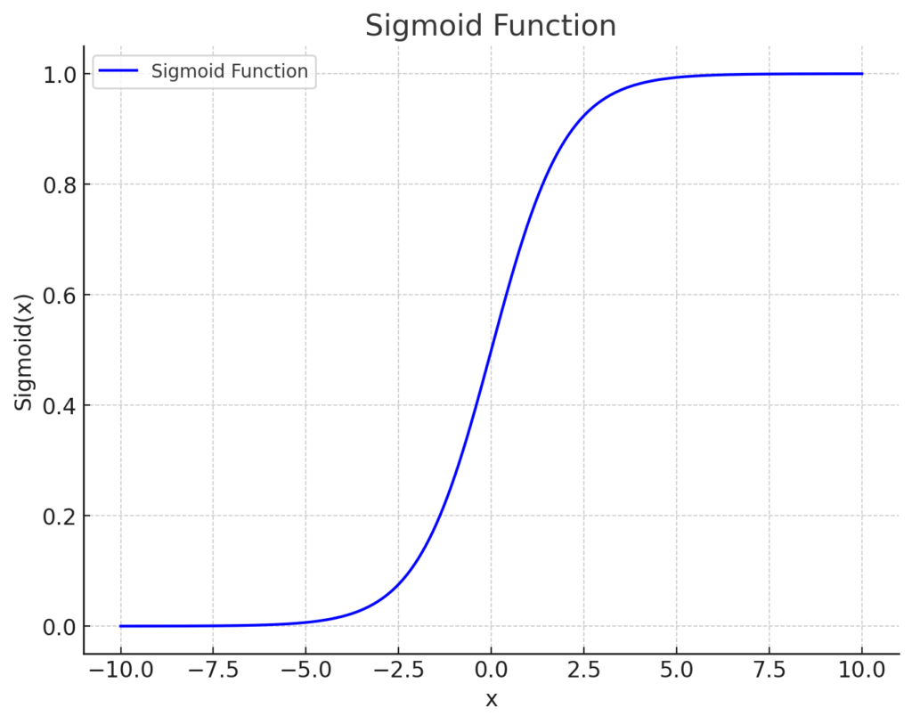
But why is this an issue? Well, let’s visualise the sigmoid function:

We can see that, as x decreases below around -5, σ(x) approaches 0, and x as increases above around 5, σ(x) approaches 1. Further changes in x beyond these values result in negligible change in σ(x). In other words, saturation occurs.
This means that if the discriminator becomes too good at identifying the generated images as fake, the feedback it provides to the generator to improve becomes less useful. Similarly, if the generator is able to out-perform the discriminator too quickly, the feedback to the discriminator uses to learn to reduce its confidence in fake images becomes less meaningful also.
More specifically, since σ(x) changes very little with respect to the change in the discriminator’s output, x, when σ(x) is close to 0 or 1, the gradient of the output with respect to the loss becomes vanishingly small—this is known as the vanishing gradient problem.
Let’s try to understand this using an example where the discriminator is strongly out-performing the generator.
1.1. Demonstration
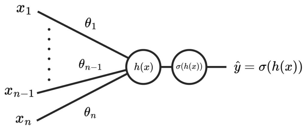
Let’s say our generator produces an image with the pixels x1, x2 … xn, which are fed to a simple discriminator network, D(x):

The discriminator is dominating, and so produces a highly negative value of h(x) = -10, giving σ(h(x)) = 0.00004 as the confidence of the image being real.
The generator’s loss for this image will be:

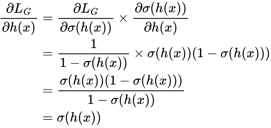
Let’s calculate the gradient ∂LG/∂h(x). To do so we work backwards from ŷ using back-propagation via the chain rule:

First we’ll calculate ∂LG/∂σ(h(x)) using the rule dloge(a)/da = 1/(1 – a):

Then ∂σ(h(x))/∂h(x) using the rule dσ(a)/da = σ(a)(1 – σ(a)):

Therefore:

This means that, whatever σ(h(x)) is, the gradient of the generator’s loss function with respect to the discriminator network’s output, ∂LG/∂h(x), will be the same. This is 0.00004 in this instance, which is very small.
To understand the effect on the generator’s learning we need to visualise the full gradient flow from LG to the generator, G(z).

To update the generator, ∂LG/∂θGi, where θGi is the i-th parameter in the generator, must be calculated. This is calculated using back-propagation from ∂LG/∂h(x) via the chain rule:

As we can see, a small ∂LG/∂h(x) causes the gradient of the loss with respect to each parameter in the generator, ∂LG/∂θGi, to be small also, due to multiplication by ∂LG/∂h(x). This means the generator won’t improve, since updates to the generator’s parameters via gradient descent will be minimal:

2. Mode Collapse
If the generator improves too quickly, or the discriminator is too weak, mode collapse can occur. Mode collapse is characterised by a break down in the diversity of images produced by the generator. This can be a limited set of images, or, In the worst case, the same image, regardless of the input noise vector, z.
This happens because the generator essentially overfits to the discriminator. The discriminator learns a set of features that it uses to distinguish real images from fake ones. If the discriminator cannot keep up, the generator can learn to produce images that replicate a limited set of features that consistently fool the discriminator. Let’s imagine that there is an image X* = G(z) that the discriminator will assign the highest confidence to, thus provides the minimum loss in LG.

If the discriminator fails to compete with the generator, the generator will gradually converge to output images that mimic optimal image X* for the full distribution of z.
Likewise, because the discriminator is assigning a high likelihood of the generated images being real, the generator’s loss will be very small. Therefore the generator will halt exploration and settle on the same set of images, or singular image.
3. An Uncertain Discriminator
If the discriminator is too weak, it may lose its ability to distinguish between real and fake images with confidence. This is characterised by a confidence that hovers around 0.5, with a lacking disparity between real and fake images. As a result, the discriminator fails to provide adequate feedback, akin to when the discriminator is dominating (Section 1).
As discussed in Section 1, the generator relies on the gradient ∂LG/∂θGi to improve itself. ∂LG/∂θGi describes the change in LG as each parameter, θGi, changes. As we’ve know, LG is:

If the discriminator always outputs values close to 0.5, however, no matter how we change θGi, the loss will always remain around -0.69:

Let’s try to understand this in a bit more depth with a demonstration.
3.1. Demonstration
Imagine our generator produces an image that is given a confidence of 0.498, and so LG will be -0.68912. θG1 is then bumped up by 0.1. This gives an increased confidence of 0.4982, and so LG decreases to -0.68955. The gradient LG with respect to θG1 is:

As we can see, this gradient is vanishingly small, and so the generator will not be able to learn effectively.
4. Final Words
In this article, we explored three key issues in training traditional GANs. Since then, research has primarily focussed on addressing these issues to provide more stable training processes. One notable advancement is the Wasserstein GAN (WGAN), which I explain in the next post.
Leave a Reply