Traditional GANs often suffer from poor stability during training, primarily due to the design of the discriminator and the loss functions used. If the delicate balance of competition between the generator and the discriminator is not maintained, issues such as mode collapse or vanishing gradients can arise. I cover some of the key challenges that affect traditional GANs in this article.
To address these issues, the Wasserstein GAN (WGAN) replaces the discriminator with a critic and redesigns the loss functions for both the discriminator and the generator. These changes provide more meaningful, continuous learning curves, and help to avoid vanishing gradients which can otherwise hinder generator optimisation.
1. Critic Instead of a Discriminator
The traditional discriminator uses the sigmoid function to output a confidence between 0 and 1 denoting whether the image is real. However, as discussed in this article, the sigmoid function, σ(x), saturates at 0 and 1 as x becomes increasingly positive or negative. This means that the gradient of σ(x) with respect to x will become vanishingly small if the confidence is close to 0 or 1 and training will fail.
The critic solves issues of unstable training by removing the sigmoid function. As a result, the output C(G(z)) is no longer a confidence bounded between 0 and 1, but rather a real, unbounded value that denotes a numerical score of how real the image is.
Of course, this means the Binary Cross Entropy (BCE) loss can no longer be used, so the loss functions for the critic and generator must change. These adjustments are implemented by the Wasserstein Loss.
2. Wasserstein Loss
The critic outputs a numerical score of how real the image is that can be positive or negative, and any magnitude (but this is limited indirectly by weight clipping or a gradient penalty, which will be discussed later).
The goal of the critic is to assign a higher score to real images and a lower score to fake images from the generator. In other words, the critic’s goal is to maximise the difference in C(x) and C(G(z)), where C(x) is the critic’s score for real images and C(G(z)) is the score for fake ones:

This is referred to as the earth mover’s distance. To understand why, imagine we plot the distribution of scores assigned to our fake images and the scores assigned to our real ones:
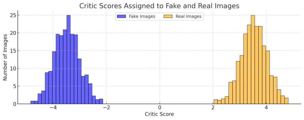
(This graph is often represented using a continuous line for the probability distribution; for simplicity, it is shown here as a quantised histogram).
The goal of the discriminator is to move the distribution of fake images and the distribution of real images apart. This is called the earth mover’s distance because, by analogy, it is akin to finding the distance required (the cost) to move two mounds of earth (dirt) together.
The discriminator’s task is to maximise this distance, but gradient descent can only minimise a given loss function. Instead, we can minimise the negative of the earth mover’s distance:

By minimising the negative of the earth mover’s distance, this has the same effect as maximising it.
2.1. Critic Loss Demonstration
We retrieve a real image from our dataset and feed it to the critic. We also generate a fake image using the generator, and feed this to the critic.
The critic scores the real image 2.7 and the fake one -3.1, and so the loss is:
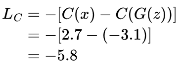
We can see that the loss is allowed to become increasingly negative, rather than being bounded at 0. A loss of 0 is happens when the critic assigns the same score to real images as it does fake ones; a positive loss means the critic is assigning a higher score to fake images.
In other words, the loss should always be negative for a critic that is performing as intended.
2.2. New Generator Loss
To generate realistic images, the generator’s task is to improve itself by maximising the score given to its generated images, C(G(z)), by the critic.
As discussed previously, gradient descent can only minimise a loss function, and so we minimise the negative of C(G(z)) for the loss function:

3. Weight Clipping
The critic’s score is unbounded and can take on any value. Combined with the fact that the optimal loss converges to negative infinity, this can lead to issues such as increasingly large gradients, ultimately resulting in gradient explosion. One approach to prevent the critic’s score from becoming too large is to apply weight clipping.
Weight clipping limits the magnitude of the weights, which in turn limits the gradient of the critic’s output with respect to its input values. Precisely, the goal is to limit the gradient to 1-Lipschitz; this means that the L2 norm of the gradient is less than or equal to 1 for all inputs:

In practice, however, the goal is to keep the L2 norm of the gradient close to 1, because if the norm becomes too small, it can hinder the critic’s ability to learn effectively.
To apply weight clipping, each weight is simply clamped between an upper and lower bound every time it is updated:

The values of cmin and cmax used in WGAN’s original paper were -0.01 and 0.01, respectively.
While weight clipping improves training stability, it can also lead to underfitting of the critic, since its capacity to capture relationships in real and fake images is constrained. Additionally, cmin and cmax require tuning to achieve a 1-Lipschitz gradient, and this tuning depends on the network architecture.
4. Gradient Penalty (WGAN-GP)
Similar to weight clipping, the gradient penalty aims to enforce the 1-Lipschitz constraint, but without restricting the values of the weights. Instead, it adds a penalty to the loss function that encourages the network to constrain its gradient within 1-Lipschitz. In other words, any deviation of the L2 norm of the gradient from 1 is penalised. The new loss function is, therefore:

The gradient penalty here is the term:

Let’s try to break down this equation. First, λ is a hyperparameter that controls the impact of the deviation from 1-Lipschitz on the overall loss. A high λ means that a high level of focus will be placed on keeping the gradient within 1-Lipschitz. In the original paper, λ is set to 10.
x̂ is perhaps the most interesting part of this equation. Recall how earlier we said that for our network to be 1-Lipschitz continuous, the “L2 norm of the gradient is less than or equal to 1 for all inputs“? Well, here x̂ is a randomly chosen, interpolated point between our fake and real images. By doing so, we can ensure that the 1-Lipschitz constraint is maintained across all possible input values.

x̂ is essentially a real image sampled from the dataset that is blended with a fake image from the generator. The amount of each image is defined by ε, the value of which is a randomly-sampled, real number value between 0 and 1.
4.1. Demonstration
Let’s say we have a dataset of 3×3 grayscale images, and we sample a real image x from the dataset and generate a fake image G(z) from the generator:
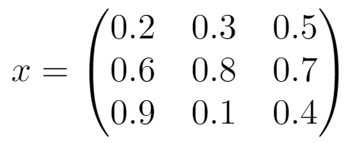
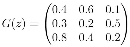
ε is assigned a random value of 0.31, and so x̂ is:
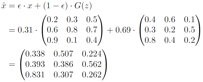
x̂ is then fed into the critic to give C(x̂) = -2.1.
The gradient of this output with respect to each input pixel is then computed. For our critic at the current stage of training, these values happens to be:

We then calculate the L2 norm of the gradients:

Finally, using λ = 10, we can calculate the gradient penalty:
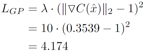
When this penalty is added to the critic’s loss, gradient descent will encourage the critic to adapt its weights so that the L2 norm of the gradients is closer to 1.

Leave a Reply