The core principle of model-based machine learning is the optimisation process, which allows algorithms to learn. The cost function quantifies the error of the current algorithm, and optimiser modifies the algorithm by some degree to reduce that error; this gradual movement towards the (local) minimum error is called “convergence”.

In ML algorithms that model a mathematical relationship between input features and output features, optimisation is typically performed using a form of gradient descent. In this article, I will be demonstrating gradient descent for linear regression.

1. Understanding the Problem

Let’s consider the following datapoints:

x	0	1	2	3
y	1	3	5	y3

The task is to produce an algorithm that learns the mathematical relationship that maps x -> y, and then, using this model, predict what y₃ will be.

We can see that this relationship y = 2x + 1, and so y₃ should be 7. But how could machines learn this relationship? Well, let’s compose this problem algebraically:

Given y = θ₁x + θ₀, we want to find the values for θ₀ and θ₁ that, for each x value, gives us the closest predicted y value (ŷ) to the target y value (y).

2. Cost Function

To start with, we will initialise θ₀ and θ₁ to any small value:

Let θ₀ = 0.5

Let θ₁ = 0.5

Using y = 0.5x + 0.5, we obtain the following predicted y values (ŷ) for each x:

x	0	1	2	3
y	1	3	5	y3
ŷ	0.5	1	1.5	2

We can better visualise this on a graph:

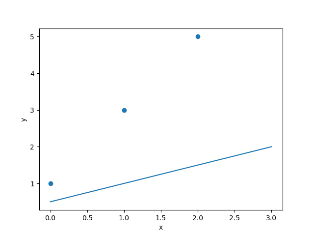
The blue line is our current function y = 0.5x + 0.5, and the blue dots represent our target values.

To quantify the error, one might think of adding up all the differences between each predicted y (ŷ) and target y:

However, if we did this, the error would increase as we have more data points (x values). Therefore, we divide the error by the number of data points, n.

But what if (y – ŷ) isn’t always positive? If we have (2 – 4) + (4 – 2), we will get an error of -2 + 2 = 0, but we should get an error of 2 + 2 = 4. Well, we can use the absolute difference instead:

What we have created here is the Mean Absolute Error (MAE), however, more commonly, we square (y – ŷ); this is the Mean Squared Error (MSE):

If you’re curious why we might use MAE over MSE, or vice versa, I tend to explain this in a future post.

3. Understanding Gradients

Now we can quantify the model’s error, we need to understand how to change θ₀ and θ₁ to reduce it. First, we need to know the rate of change of the MSE with respect to the change in θ₀ and θ₁. To do so, we calculate the gradient of the MSE with respect to θ₀ and θ₁ using differentiation.

If you’re familiar with differentiation, you can skip to Section 4, otherwise, let’s try to understand differentiation intuitively.

Picture a side view of yourself walking down a hill:

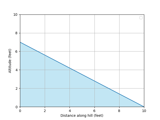
For each foot we walk along the hill, we decrease in altitude by a certain number of feet. We want to work out the rate at which we increase or decrease in altitude as we walk along the hill; this is the “gradient”, or “slope”.

If we walked from 0 foot to 10 foot along the hill, we would have decreased from 7 foot in altitude to 0 foot. Therefore, for every foot moved along the hill, our altitude changes by -7/10 = -0.7 feet. So -0.7 is our gradient. Notice that the gradient is negative. This tells us that, as we increase D, A decreases. This is important to remember when we discuss gradient descent later on.

Mathematically, the gradient is denoted as:

Δ is the delta symbol, which refers to the “change” in a variable. So ΔA is the change in altitude, A, and ΔD is the change in distance along the hill, D.

But what if our hill isn’t a straight slope?

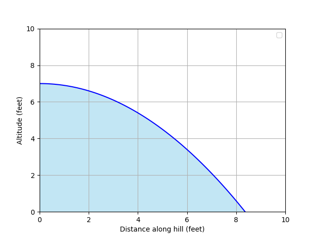
Now, for every foot we move along the hill, the rate at which our altitude is decreasing is changing. To start with, we can see that our altitude is decreasing quite slowly, but begins to decrease faster as we move further along.

So, rather than calculating the gradient for the whole hill, we can summarise the hill as the gradient at each point as we walk along it.

But if the line is curved, how do we calculate the gradient anywhere along it? Well, we can approximate the slope as a number of straight lines. This is allows us to calculate the gradient like we did before:

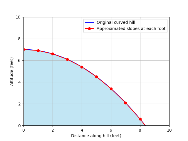
At 4 foot along the hill, our line approximation looks like this:

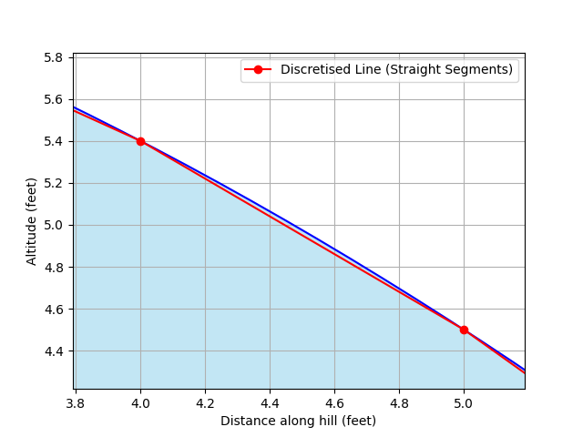
And so we can calculate the gradient at 4 foot like we did before, using this line approximation:

This gives us a gradient of -0.9 for the hill at the point where we are at 4 foot along it (D = 4).

This, however, could be more accurate. But how can we make it more accurate?

We can simply approximate the straight line over a smaller distance. For instance, rather than calculating the gradient over 1 foot from the current point, we can calculate the gradient across 0.1 foot:

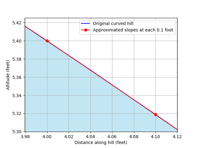
The difference between our straight line approximation and the original curve is now almost indistinguishable by eye. If we calculate the gradient of our new slope:

Our gradient is now -0.81, which is more accurate than our previous calculation of -0.9.

As we can see, as we calculate our gradient over a smaller and smaller change in the distance along the hill (ΔD), the closer our gradient will be to the real value. And so, what if this change could be infinitely small? Well, it can. This is where differentiation comes in.

3.1. Differentiation

Using differentiation, we can use an infinitely small change to calculate the gradient at any point along our function.

First, we need to know the mathematical relationship between altitude (A) and distance along the hill (D). This is A = 7 – 0.1D²

If we combine our current method of calculating the gradient, and this equation for A with respect to D, we can say that the gradient is:

If we use our previous example where D = 4 and ΔD = 0.1 we get a gradient of -0.81 just like before:

But rather than using ΔD = 0.1, we want ΔD to be as small as possible so our gradient is as accurate as possible. To do so, we want ΔD to approach 0. This is denoted using “lim”, short for “limit”. You’ll also notice that Δ changed to d; this is because d denotes an infinitely small change (an “infinitesimal difference”):

We first need to divide by ΔD, but to do so, we will have to expand (D + ΔD)² so we can isolate all the ΔD terms.

To calculate (D + ΔD)², we multiply each term in (D + ΔD) by itself and add them together. This is best demonstrated using a grid:

	D	+ΔD
D	D2	+DΔD
+ΔD	+DΔD	+ΔD2

After adding each term above, we get (D + ΔD)² = D² + 2DΔD + ΔD², which we will replace (D + ΔD)² with in our equation:

Let’s also expand some more brackets and further simplify the numerator (the top of the fraction):

Having expanded and simplified the numerator, we can now easily divide by ΔD:

Finally, we approach ΔD to 0. As you can imagine, as ΔD approaches 0, 0.1ΔD will become extremely (infinitesimally) small, so small that we can say that 0.1ΔD will be essentially 0. Therefore, we cancel the 0.1ΔD term out, giving us:

This is our final equation and is the derivative of A = 7 – 0.1D². This equation allows us to calculate the current gradient at any distance along the hill (D). If we try our previous example where D = 4:

Previously, we got a gradient of -0.81 at D = 4 using our straight line approximation.

In this section, you have learned differentiation from first principles. While providing a good understanding of how differentiation works, in practice, derivatives are rarely calculated this way. Instead, various techniques, such as the power rule, chain rule, product rule, and others, are normally used to avoid all this manual working.

4. Gradient of the Cost Function

Now you have a solid understanding of calculating the gradient, and how it tells us the rate of change of one variable with respect to another, we can apply this to gradient descent.

To know how to change θ₁ and θ₀, we need to calculate the rate of change of the MSE with respect to θ₁ and the rate of change of the MSE with respect to θ₀. Based on the previous section, you may think this is denoted as:

However, unlike in the previous section, where we had just one variable, D, that effects A, we have two variables that effect the MSE: θ₁ and θ₀. This means we are calculating the partial derivative rather than the derivative, since we have two variables but we are only calculating the derivative for one at a time (hence “partial”). This requires a different notation:

If you recall from the first section, our output prediction is calculated as ŷ = θ₁x + θ₀. If we change θ₀ by some small value, Δθ₀, our prediction will be ŷ = θ₁x + (θ₀ + Δθ0).

To find the change in MSE based on this change in θ₀, we will substitute our equations for ŷ before and after changing θ₀ into the MSE.

MSE before the change in θ₀:

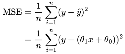
MSE after the change in θ₀:

So, using our knowledge of differentiation, we can find the rate at which the MSE changes with respect to θ₀, and in which direction (increase or decrease) using differentiation:

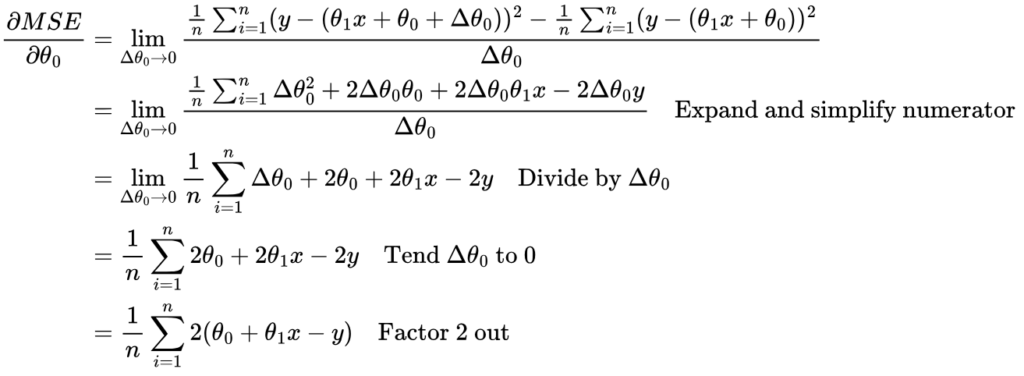
Since ŷ = θ₁x + θ₀, we can replace θ₀ + θ₁x with ŷ:

This is also sometimes written as:

Repeating this for the change in MSE with respect to the change in θ₁:

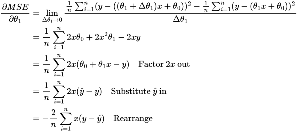
However, rather than calculating the derivative like this, the chain rule is typically used; this provides a trick that avoids all this manual working.

5. Optimisation

Let’s revisit our earlier example:

x	0	1	2	3
y	1	3	5	y3

We initialised θ₀ and θ₁ to 0.5, which gave us the predictions:

x	0	1	2	3
y	1	3	5	y3
ŷ	0.5	1	1.5	2

Now we know how to calculate the rate of change of the MSE as we change θ₀ and θ₁, we can work out what direction to change them to decrease the MSE for each prediction.

Let’s calculate the gradient of the MSE with respect to θ₀ for our initial values of θ₀ and θ₁:

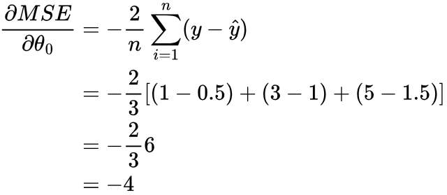
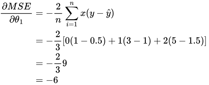
We can see that both gradients are negative; this means that as we increase θ₀ or θ₁, the MSE decreases. So, to improve how our model is performing, we need to increase θ₀ and θ₁. We already know this, since we know θ₀ should be 1 and θ₁ should be 2.

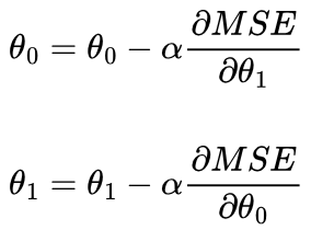
α controls how much we update θ₀ or θ₁ by. If we used α = 1, we would add 6 to θ₁, and therefore overshoot the best θ₁ of 2, and similarly for θ₀. Instead, we could choose a value of α = 0.05:

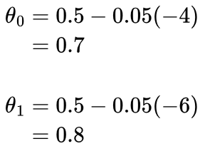
The calculation of MSE and updating of parameters θ₀ and θ₁ is one “training iteration”. We will repeat this process 200 times.

Second Iteration

ŷ = 0.8x + 0.7

x	0	1	2	3
y	1	3	5	y3
ŷ	0.7	1.5	2.3	3.1

Calculate the gradient of the MSE with respect to θ₀ and θ₁:

Update θ₀ and θ₁ in the direction that reduces MSE:

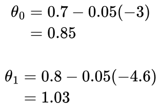
We can see that θ₀ and θ₁ are gradually moving towards their optimal values of 1 and 2, respectively.

Final Model

After repeating the training iteration 200 times, we end up with θ₀ = 1.00133 and θ₁ = 1.99904, which are very close to the actual values of 1 and 2.

Therefore the mathematical relationship that maps x -> y that has been learned is ŷ = 1.99904x + 1.00133

We can then predict what y₃ will be using ŷ = 1.99904(3) + 1.00133 = 0.699845

Our final predictions are therefore:

x	0	1	2	3
y	1	3	5	y3
ŷ	1.00133	3.00037	4.99941	6.99845

But what really happened? Let’s picture how the MSE changes as θ₀ and θ₁ change on a graph.

5.1. Gradient Descent Visualisation

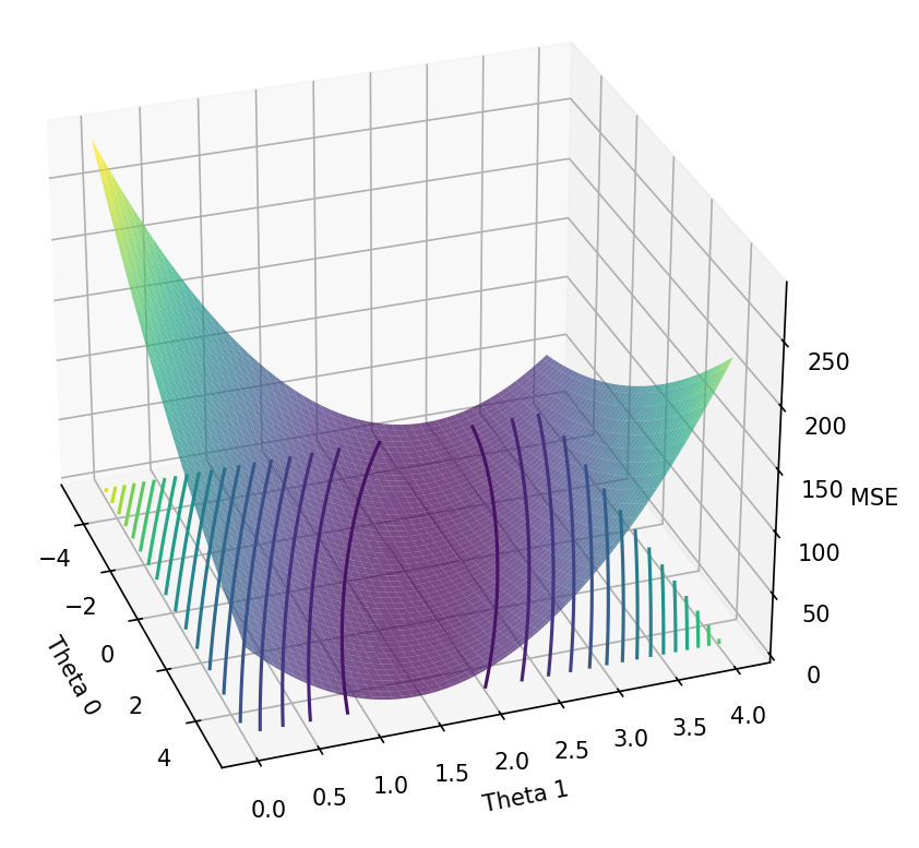
The above graph shows values of MSE as θ₀ and θ₁ change. This visualisation can be referred to as the “loss landscape”. The goal is to descend down to the lowest point, where the MSE (error) is the lowest. This can be thought of as traversing down a hill, where the MSE is the altitude and θ₀ and θ₁ are our coordinates. At each point along the hill, we assess what direction to move in that is the steepest, then change our coordinates (θ₀ and θ₁) in that direction.

6. Stochastic Gradient Descent

Stochastic Gradient Descent (SGD) is the most commonly used implementation of gradient descent. Rather than calculating the gradient of the MSE with respect to θ₀ and θ₁ for all datapoints, this is calculated for a single datapoint or mini-batch of datapoints. In other words, we divide the datapoints up into groups, which we perform a training iteration for separately. We do this since datasets often contain large numbers of datapoints, which makes calculating the gradient across all datapoints at once too inefficient.

Additionally, this is how training iterations differ to epochs. Epochs are the number of times the training is performed for the whole dataset, whereas training iterations are often performed multiple times per epoch, based on the number of groups of data points (the batch size).